Initial conditions

Two initialization modes are available, selected via INITFLG in srjob.sh (see Submit a job):

Restart run (INITFLG=""): the model continues from HYCOM and CICE restart files valid at the start date. This is the standard mode for hindcast and forecast runs. See Restart files below for how to obtain them.
Climatological initialization (cold start, INITFLG="--init"): temperature and salinity (T/S) are read from relax/<IEXPT>/relax_tem.[ab] and relax_sal.[ab]; layer thicknesses are computed internally from the T/S profiles; velocities and sea surface height (SSH) start at zero. The start date must be in September (Arctic sea ice is at its annual minimum in September, making it a natural starting point). The ice state is initialised from a climatology derived from TP4 assimilation data (TP4b_1991-2020_AssimSurf.nc); the same source is used for both TP2 and TP5. Expect a multi-year spin-up before the circulation is reliable. See Climatologies and river forcing for how to prepare the required files.

Note

The relax_* file names reflect their use as targets for climatological relaxation during the run (see Climatologies and river forcing). During initialization, no relaxation is applied. The files are simply read once as the initial T/S state.

Restart files

HYCOM and CICE each need a restart file valid at the start date of the run (consistent with START in the srjob.sh variable table). The naming conventions are as follows:

Model	File	Notes
HYCOM	`restart.YYYY_DDD_00_0000.[a,b]`	`DDD` is the three-digit day of year (zero-padded)
CICE	`iced.YYYY-MM-DD-00000.nc`	Standard calendar date

Warning

HYCOM 2.3 restart files are not compatible with HYCOM 2.2. If you have restart files produced by a 2.3 run, you cannot use them to restart a 2.2 model. The reverse is fine: 2.2 restart files can be used to start a 2.3 run. The archived restart files below come from HYCOM 2.3.

For TP2 hindcast runs, restart files are archived at:

/nird/datalake/NS9481K/shuang/TP2_output/expt_02.6/

For example, to start on 27 August 2016 (240th day of year):

EXPT_ID=<EXPT_ID>         # e.g. 01.0

mkdir -p $WDIR/expt_${EXPT_ID}/data/cice
cd $WDIR/expt_${EXPT_ID}/data

cp /nird/datalake/NS9481K/shuang/TP2_output/expt_02.6/restart/restart.2016_240_00_0000.a .
cp /nird/datalake/NS9481K/shuang/TP2_output/expt_02.6/restart/restart.2016_240_00_0000.b .

cd cice
cp /nird/datalake/NS9481K/shuang/TP2_output/expt_02.6/cice/iced.2016-08-27-00000.nc .

Atmospheric forcing

This step is handled by the script atmo_synoptic.sh.

Note

The job script srjob.sh calls atmo_synoptic.sh automatically (see Submit a job). Skip this section if you submit via srjob.sh (recommended). You may still want to run atmo_synoptic.sh manually to verify the input files are in place before submitting; if so, comment out the atmo_synoptic.sh call in srjob.sh to prevent the job from regenerating the files (output filenames have no dates, so they would be silently overwritten).

Atmospheric forcing must be prepared for each run period. START and END are the run start and end times, see the srjob.sh variable table for the expected format. To prepare it manually, first activate the Python environment, then run:

CONFIGNAME=<CONFIGNAME>   # e.g. TP2a0.10
EXPT_ID=<EXPT_ID>         # e.g. 01.0

cd $WORK/${CONFIGNAME}/expt_${EXPT_ID}
$HOME/NERSC-HYCOM-CICE/bin/atmo_synoptic.sh era5+lw $START $END

Running atmo_synoptic.sh creates the following files under $WORK/<CONFIGNAME>/force/synoptic/<IEXPT>/:

File	Contents
`airtmp.[ab]`	2 m air temperature
`dewpt.[ab]`	2 m dew point temperature
`mslprs.[ab]`	Mean sea level pressure
`precip.[ab]`	Total precipitation rate
`radflx.[ab]`	Net longwave radiation at the surface
`shwflx.[ab]`	Downwelling shortwave radiation
`vapmix.[ab]`	Water vapour mixing ratio
`wndewd.[ab]`	Eastward (u) wind component at 10 m
`wndnwd.[ab]`	Northward (v) wind component at 10 m

Since output goes to an experiment-specific directory (force/synoptic/<IEXPT>/), running atmo_synoptic.sh from different experiments within the same configuration will not cause conflicts.

Since forcing files do not include dates in their filenames, atmo_synoptic.sh automatically creates a stamp file in the output directory recording the period covered, e.g. stamp_2013-01-01T00:00:00-2013-01-05T00:00:00. The file is empty: the date range is encoded in the filename.

Open boundary forcing

The open boundaries of a regional ocean model must be forced by time-varying fields (e.g., temperature, salinity, velocity, and optionally BGC tracers) from an external ocean product. The source can be a reanalysis such as GLORYS12 or output from another ocean model simulation that covers the domain boundaries. This approach is called offline nesting, and is the approach supported by NERSC-HYCOM-CICE: information flows in one direction only, from the external product into the regional model. The regional model has no influence on the boundary conditions it receives. This is in contrast to online (two-way) nesting, where the regional model (the inner nest) and an outer nest model run simultaneously and exchange information at their shared boundary. Online nesting is not supported here. Further detail on offline nesting in HYCOM can be found in the HYCOM User Guide and the HYCOM examples wiki.

Offline nesting is activated in HYCOM-CICE by setting nestfq > 0 (interval in days between 3D nesting archive reads) or bnstfq > 0 (interval in days between barotropic nesting archive reads) in blkdat.input. Three groups of files are required:

Boundary configuration files — define the open boundary geometry and relaxation coefficients for the boundary nudging zone (ports.input, rmu, rmutr).
Nesting files — pre-interpolated boundary conditions from the external product, stored in HYCOM’s archv format. Must span the run period; HYCOM interpolates in time between snapshots.
Sponge layers (optional) — spatially varying biharmonic diffusion fields (thkdf4, veldf4) that damp noise near the open boundaries.

Boundary configuration files

The following files must be present under $WORK/<CONFIGNAME>/nest/<IEXPT>/:

File	Contents
`ports.input`	Open boundary section definitions
`rmu.a` / `rmu.b`	2D relaxation coefficient field for physics nudging at open boundaries
`rmutr.a` / `rmutr.b`	2D relaxation coefficient field for BGC tracer nudging at open boundaries

For TP2, you can copy these files from the following reference experiment:

CONFIGNAME=<CONFIGNAME>   # e.g. TP2a0.10
IEXPT=<IEXPT>             # e.g. 010

DIR_NST=/nird/datalake/NS9481K/shuang/nest/TP2_expt023
mkdir -p $WORK/${CONFIGNAME}/nest/${IEXPT}
cd $WORK/${CONFIGNAME}/nest/${IEXPT}
cp ${DIR_NST}/ports.input .
cp ${DIR_NST}/rmu.a ${DIR_NST}/rmu.b .
cp ${DIR_NST}/rmutr.a ${DIR_NST}/rmutr.b .

Open boundary sections (ports.input)

Each port in ports.input defines one open boundary segment. The file lists nports followed by five values per port:

Field	Description
`kdport`	Orientation: `1`=N, `2`=S, `3`=E, `4`=W
`ifport`	First i-index of the boundary segment
`ilport`	Last i-index (`= ifport` for N or S boundaries)
`jfport`	First j-index of the boundary segment
`jlport`	Last j-index (`= jfport` for E or W boundaries)

For N/S boundaries the segment spans a range of i-indices at a fixed j; for E/W boundaries it spans a range of j-indices at a fixed i.

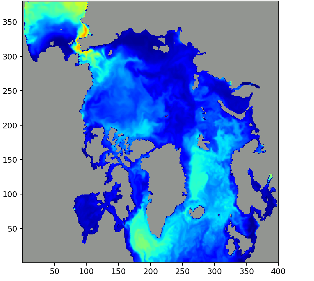
TP2 domain (400×380 grid). Gray areas are the land mask. The two open boundaries are the Pacific boundary (past the Bering Strait, northern edge) and the Atlantic boundary (southern edge). Technically a third open boundary exists at the western portion of the northwest corner, but it has been closed (set to land) for simplicity — visible as a small stripe of land in the figure.

Example ports.input for TP2 (two open boundary passages):

'nports'
'kdport'   5  'ifport'   102  'ilport'   380  'jfport'   380  'jlport'
'kdport'   174  'ifport'  348  'ilport'     2  'jfport'     2  'jlport'

Port 1 (kdport=1, North): along the northern edge of the domain (j=380), spanning the western portion of the grid (i=5–102). This is the Pacific open boundary, past the Bering Strait.
Port 2 (kdport=2, South): along the southern edge of the domain (j=2), spanning the central portion of the grid (i=174–348). This is the Atlantic open boundary.

At these boundaries the model reads fields like temperature, salinity, and velocity from the parent model and relaxes toward them according to the rmu field.

Nesting files

HYCOM uses archv files as its standard model state snapshot format: each file stores the full model state (3D fields such as temperature, salinity, velocity, and layer thickness, plus 2D fields such as sea surface height and Montgomery potential) at a single point in time on the model grid and hybrid vertical coordinate system. In the nesting context, the same format is used for the pre-interpolated boundary conditions from the external product. The fields cover the entire inner model domain (not just the boundary cells) because nudging is applied volumetrically over the boundary nudging zone defined by nest/rmu.

HYCOM reads a new archive at the interval set by nestfq (or bnstfq) and interpolates in time between consecutive snapshots. For TP2, daily files are used. These files must be present in $WORK/<CONFIGNAME>/nest/<IEXPT>/, covering the full run period. The expected file names are:

File	Contents
`archv.YYYY_DDD_HH.a` / `.b`	Physics boundary conditions (`DDD` = zero-padded day of year, `HH` = hour, typically `00`)
`archv_fabm.YYYY_DDD_HH.a` / `.b`	BGC boundary conditions (only needed when running with FABM)

Nesting files for TP2 are archived at /nird/datalake/NS9481K/shuang/nest/TP2_expt023/. Use stage_nesting_files.sh to copy or extract the files needed for a given date range:

CONFIGNAME=<CONFIGNAME>   # e.g. TP2a0.10
IEXPT=<IEXPT>             # e.g. 010

$HOME/NERSC-HYCOM-CICE/bin/stage_nesting_files.sh \
    /nird/datalake/NS9481K/shuang/nest/TP2_expt023 \
    $WORK/${CONFIGNAME}/nest/${IEXPT} \
    <START> \
    <END>

Here, START and END are the run start and end times, see the srjob.sh variable table for the expected format. Two optional flags are supported (in any order):

Flag	Effect
`--no-fabm`	Skip BGC (FABM) archive files
`--skip-existing`	Skip dates where all expected files are already present in the destination directory

Note

The archived TP2 nesting files have montg1 set to a non-zero value, but it may have been computed from a different model run than the restarts you are using. Always run the Montgomery potential correction step below to ensure consistency.

Generating nesting files from GLORYS12/CMEMS

For TP2, pre-generated files are available at the path above. If you need to generate nesting files from scratch (for a different time period, source product, or configuration) use the workflow below. Two products from the Copernicus Marine Environment Monitoring Service (CMEMS) are used as source data, both on a regular lat/lon grid:

Physics: GLORYS12 reanalysis (CMEMS GLOBAL_MULTIYEAR_PHY_001_030)
BGC: CMEMS global ocean biogeochemistry reanalysis (GLOBAL_MULTIYEAR_BIO_001_033) or near-real-time forecast (GLOBAL_ANALYSIS_FORECAST_BIO_001_029)

Step 0 — Copy source region files (once)

The source region directory NMOb0.08/ needs two things in place before any step can run:

NMOb0.08/REGION.src, NMOb0.08/expt_01.0/ (including blkdat.input) — these are part of the repository.
NMOb0.08/topo/ — grid and bathymetry files that are too large for the repository. Both Step 1 and Step 2 read from this directory, so copy them once from NIRD:
```
cp -r /nird/datapeak/NS9481K/MERCATOR_DATA/NMOb0.08/topo \
    $HOME/NERSC-HYCOM-CICE/NMOb0.08/
```

Step 1 — Create interpolation matrix (once per source/destination pair)

This step reads the grid coordinates of both the source (GLORYS12) and destination (HYCOM) regions and uses a conjugate gradient method to find, for each point on the destination grid, the corresponding fractional indices on the source grid. The result is a mapping array stored in gmap.[ab] that Step 2 uses to horizontally interpolate every field. This step only depends on the grid geometry, not the ocean fields, so it only needs to be run once per source/destination grid pair.

CONFIGNAME=<CONFIGNAME>   # e.g. TP2a0.10

cd $HOME/NERSC-HYCOM-CICE/NMOb0.08/expt_01.0
$HOME/NERSC-HYCOM-CICE/bin/isuba_gmapi.sh $WORK/${CONFIGNAME}/

isuba_gmapi.sh is a bash script that calls a compiled Fortran binary in $HOME/NERSC-HYCOM-CICE/hycom/hycom_ALL/hycom_2.2.72_ALL. No Python environment is needed. If you followed the compilation guide, the binary will already be in place.

Output: $HOME/NERSC-HYCOM-CICE/NMOb0.08/subregion/TP2a0.10.gmap.[ab]

Step 2 — Interpolate fields

nemo_to_hycom.sh horizontally and vertically interpolates the external fields onto the HYCOM grid and hybrid vertical coordinate, and accepts the following options:

Option	Description
`-d`	Destination experiment path (mandatory)
`-n`	Path pattern of physics input NetCDF files (mandatory)
`-g`	Source grid type; always set to `regular` for current GLORYS12 and BGC products
`-b`	BGC input path pattern; also activates BGC boundary creation (optional)
`-i`	Search radius for wet-point lookup (optional, default: 50 grid cells)
`-m`	Path to the GLORYS12 mesh file (contains grid, bathymetry, mask) (mandatory for `-g regular`)
`-c`	Path to the GLORYS12 coordinates file (contains vertical layer thicknesses `e3t`) (mandatory for `-g regular`)
`-h`	Print usage information and exit

The GLORYS12 and BGC files on NIRD follow these naming conventions:

Physics (-n): MERCATOR-PHY-24-YYYY-MM-DD-12.nc (one file per day, timestamped at 12:00 UTC)
BGC (-b): global_analysis_forecast_bio_YYYYMMDD.nc (one file per day)

Note

BGC tracers are interpolated onto the vertical layer structure derived from the physics fields and must be processed together in a single pass. -n and -b must always cover the same date; the script does not verify this, so make sure they match.

nemo_to_hycom.sh calls both a Python script and a compiled Fortran binary. Before running, load the HPC environment and activate the Python environment:

In the examples below, omit -b for physics-only runs.

Single day (2018-01-01), from the login node:

CONFIGNAME=<CONFIGNAME>   # e.g. TP2a0.10
EXPT_ID=<EXPT_ID>         # e.g. 01.0

cd $HOME/NERSC-HYCOM-CICE/NMOb0.08/expt_01.0
$HOME/NERSC-HYCOM-CICE/bin/nemo_to_hycom.sh \
    -d $WORK/${CONFIGNAME}/expt_${EXPT_ID}/ \
    -n "/nird/datapeak/NS9481K/MERCATOR_DATA/PHY/2018/MERCATOR-PHY-24-2018-01-01-12.nc" \
    -g regular \
    -b "/nird/datapeak/NS9481K/MERCATOR_DATA/BIO/DAILY/2018/global_analysis_forecast_bio_20180101.nc" \
    -m "/nird/datapeak/NS9481K/MERCATOR_DATA/REGULAR_GRID_COORD/GLO-MFC_001_030_mask_bathy.nc" \
    -c "/nird/datapeak/NS9481K/MERCATOR_DATA/REGULAR_GRID_COORD/GLO-MFC_001_030_coordinates.nc"

Processing a single day takes approximately 20 minutes on the login node, which is pretty slow. For multi-day, multi-month or multi-year runs, use a compute node to perform Step 2.

Compute nodes on Betzy cannot access NIRD, so source files must be copied to $WORK from the login node first. Set START and END to your period, then run the following. PHY and BIO are copied in parallel (& runs a command in the background; wait blocks until both finish before moving to the next year):

START=2018-01-01
END=2018-01-31

DATE=$START
while [[ $(date -d "$DATE" +%s) -le $(date -d "$END" +%s) ]]; do
    YYYY=$(date -d "$DATE" +%Y)
    YYYYMMDD=$(date -d "$DATE" +%Y%m%d)
    mkdir -p $WORK/input/GLORYS12/PHY/${YYYY}
    mkdir -p $WORK/input/GLORYS12/BIO/${YYYY}
    rsync -av \
        /nird/datapeak/NS9481K/MERCATOR_DATA/PHY/${YYYY}/MERCATOR-PHY-24-${DATE}-12.nc \
        $WORK/input/GLORYS12/PHY/${YYYY}/ &
    rsync -av \
        /nird/datapeak/NS9481K/MERCATOR_DATA/BIO/DAILY/${YYYY}/global_analysis_forecast_bio_${YYYYMMDD}.nc \
        $WORK/input/GLORYS12/BIO/${YYYY}/ &
    wait
    DATE=$(date -d "$DATE + 1 day" +%Y-%m-%d)
done
mkdir -p $WORK/input/GLORYS12
rsync -av \
    /nird/datapeak/NS9481K/MERCATOR_DATA/REGULAR_GRID_COORD/GLO-MFC_001_030_mask_bathy.nc \
    /nird/datapeak/NS9481K/MERCATOR_DATA/REGULAR_GRID_COORD/GLO-MFC_001_030_coordinates.nc \
    $WORK/input/GLORYS12/

Submission script

The following script loops over all days in a year range, runs up to 12 nemo_to_hycom.sh processes in parallel, and skips dates where output already exists. The limit of 12 is memory-based: each job uses ~16 GB peak RAM, and 12 × 16 GB = 192 GB requested via --mem-per-cpu=16GB. Unlike the interactive devel session, preproc bills only for the resources requested rather than a full node, making it more economical for longer runs. Copy source files from the login node as described above before submitting.

Submit the job

Save the script below as nesting_job.sh in $WORK/<CONFIGNAME>/expt_<EXPT_ID>/. Set CONFIGNAME, IEXPT, and EXPT_ID at the top of the script to match your experiment, then submit with the start and end year as arguments:

CONFIGNAME=<CONFIGNAME>   # e.g. TP2a0.10
EXPT_ID=<EXPT_ID>         # e.g. 01.0

cd $WORK/${CONFIGNAME}/expt_${EXPT_ID}
sbatch nesting_job.sh 2018 2019

#!/bin/bash
#SBATCH --job-name=nesting
#SBATCH --account=nn2993k
#SBATCH --time=24:00:00
#SBATCH --qos=preproc
#SBATCH --ntasks=12
#SBATCH --mem-per-cpu=16GB
#SBATCH -o log/nemo2hycom.%J.out
#SBATCH -e log/nemo2hycom.%J.err

source ${HOME}/NERSC-HYCOM-CICE/environment/betzy_env.sh
module load Miniforge3/24.1.2-0
source ${EBROOTMINIFORGE3}/bin/activate
conda activate hycom-cice

CONFIGNAME=<CONFIGNAME>   # e.g. TP2a0.10
IEXPT=<IEXPT>             # e.g. 010
EXPT_ID=<EXPT_ID>         # e.g. 01.0

start_year=$1
end_year=$2
if [[ -z "$start_year" || -z "$end_year" ]]; then
    echo "Usage: sbatch nesting_job.sh <START_YEAR> <END_YEAR>"
    exit 1
fi

cd $HOME/NERSC-HYCOM-CICE/NMOb0.08/expt_01.0
$HOME/NERSC-HYCOM-CICE/bin/archvz2hycom_biophys.sh --setup-only $WORK/${CONFIGNAME}/expt_${EXPT_ID}/

DATE="${start_year}-01-01"
END="${end_year}-12-31"
nproc=0
while [[ "$DATE" < "$END" || "$DATE" == "$END" ]]; do
    YYYY=$(date -d "$DATE" +%Y)
    DDD=$(date -d "$DATE" +%j)
    YYYYMMDD=$(date -d "$DATE" +%Y%m%d)
    archv="$WORK/${CONFIGNAME}/nest/${IEXPT}/archv.${YYYY}_${DDD}_00.b"
    if [ -e "$archv" ]; then
        echo "Skipping $DATE (output exists)"
    else
        $HOME/NERSC-HYCOM-CICE/bin/nemo_to_hycom.sh \
            -d $WORK/${CONFIGNAME}/expt_${EXPT_ID}/ \
            -n "$WORK/input/GLORYS12/PHY/${YYYY}/MERCATOR-PHY-24-${DATE}-12.nc" \
            -g regular \
            -b "$WORK/input/GLORYS12/BIO/${YYYY}/global_analysis_forecast_bio_${YYYYMMDD}.nc" \
            -m "$WORK/input/GLORYS12/GLO-MFC_001_030_mask_bathy.nc" \
            -c "$WORK/input/GLORYS12/GLO-MFC_001_030_coordinates.nc" &
        nproc=$((nproc+1))
        if [ $nproc -ge 12 ]; then
            wait
            nproc=0
        fi
    fi
    DATE=$(date -d "$DATE + 1 day" +%Y-%m-%d)
done
wait

The log/ directory must exist, which it does if you followed the experiment setup.

Note

nemo_to_hycom.sh writes montg1 = 0 in the output archives. Correct this as described below before using these files for a model run.

Output: $WORK/<CONFIGNAME>/nest/<IEXPT>/archv.YYYY_DDD_HH.[ab]

Fix the Montgomery potential

The nesting archives require a correct montg1 (Montgomery potential) field, which depends on psikk (the Montgomery potential at the deepest isopycnal interface) and thkk (the virtual bottom layer thickness) from a restart file of the destination model. Files generated by nemo_to_hycom.sh in the dropdown above have montg1 = 0; files copied from elsewhere may have a non-zero value but one computed from a different model run, making it inconsistent with the restart files you are using.

Run calc_montg1.py once per archive file, from the destination experiment directory. Before running, load the HPC environment and activate the Python environment:

CONFIGNAME=<CONFIGNAME>   # e.g. TP2a0.10
IEXPT=<IEXPT>             # e.g. 010
EXPT_ID=<EXPT_ID>         # e.g. 01.0

cd $WORK/${CONFIGNAME}/expt_${EXPT_ID}
mkdir -p ../nest/${IEXPT}/Montg
python $HOME/NERSC-HYCOM-CICE/bin/calc_montg1.py \
    ../nest/${IEXPT}/archv.YYYY_DDD_00.a \
    ./data/restart.YYYY_DDD_00_0000.a \
    ../nest/${IEXPT}/Montg/
mv ../nest/${IEXPT}/Montg/archv.YYYY_DDD_00.[ab] ../nest/${IEXPT}/

Replace restart.YYYY_DDD_00_0000.a with the actual restart file in data/ (see Restart files), and archv.YYYY_DDD_00.a with the nesting file whose Montgomery potential you want to modify.

The script cannot read and write the same file simultaneously, so the corrected file is written to a temporary Montg/ subdirectory and then moved back to overwrite the original. Use any restart from the same model run you will use for your simulation. All restarts from the same run produce the same montg1 because psikk and thkk do not vary within a run, so it does not matter which restart date you choose. Executing the above command takes roughly 12 seconds on a login node, so for many files consider running in parallel on a compute node using one of the options below.

Sponge layers

A common use of nesting is to add a sponge layer near the open boundaries: enhanced biharmonic diffusion that smooths the solution near the boundary. This is done by setting thkdf4 and veldf4 to negative values in blkdat.input, which tells the model to read spatially varying 2D fields from file rather than using a uniform scalar. The following files must then be present under $WORK/<CONFIGNAME>/relax/<IEXPT>/:

Note

The sponge layer (enhanced diffusion), the boundary nudging zone (nest/rmu), and the climatological relaxation zone (relax_rmu) are three independent mechanisms with independently defined spatial extents. They are generated by separate scripts and need not cover the same area.

File	Description
`thkdf4.[a,b]`	2D biharmonic diffusion coefficient for layer thickness
`veldf4.[a,b]`	2D biharmonic diffusion coefficient for velocity

Note

Spatially varying thkdf4 and veldf4 fields are not limited to sponge layers. Any spatially varying biharmonic diffusion pattern can be prescribed this way. The sponge layer is just the most common use case in a nesting context.

These files are generated as follows. First, create a scratch directory and link in the grid and topography files:

CONFIGNAME=<CONFIGNAME>   # e.g. TP2a0.10
IEXPT=<IEXPT>             # e.g. 010

mkdir -p $WORK/${CONFIGNAME}/relax/${IEXPT}/SCRATCH
cd $WORK/${CONFIGNAME}/relax/${IEXPT}/SCRATCH
ln -sf $WORK/${CONFIGNAME}/topo/regional.grid.a .
ln -sf $WORK/${CONFIGNAME}/topo/regional.grid.b .
ln -sf $WORK/${CONFIGNAME}/topo/regional.depth.a .
ln -sf $WORK/${CONFIGNAME}/topo/regional.depth.b .

Copy the script locally:

cp $HOME/NERSC-HYCOM-CICE/bin/hycom_creat_thkdf4_veldf4.py .

Open the script and set the parameters for your configuration:

Parameter	TP2	TP5	Description
`mnn`	`0.05`	`0.02`	Minimum diffusion value
`mxx`	`0.125`	`0.125`	Maximum diffusion value

Then activate the Python environment and run the script with the sponge layer width as its argument (20 grid cells for TP2):

python hycom_creat_thkdf4_veldf4.py 20

Copy the output to the parent directory:

cp thkdf4.a thkdf4.b veldf4.a veldf4.b ../

Climatologies and river forcing

This step is handled by create_ref_case.sh, which generates the files needed for climatological relaxation and climatological initialization. Climatological relaxation nudges T, S, and interface heights toward monthly climatology in a zone along selected open boundary walls. This is distinct from nesting nudging, which nudges toward time-varying GLORYS fields. The two mechanisms are independent and can operate simultaneously. The default in create_ref_case.sh activates the Pacific open boundary (the Northern wall in grid coordinates) only: 20 grid cells wide, with a 20-day e-folding time at the wall decreasing linearly to zero. The width and time scale are set in create_ref_case.sh, not in blkdat.input. relax in blkdat.input is simply an on/off switch for climatological relaxation.

create_ref_case.sh generates:

T/S and interface climatologies (relax_sal, relax_tem, relax_int) — nudging targets for climatological relaxation, and initial T/S state for climatological initialization
Climatological relaxation mask (relax_rmu) — 2D field of 1/e-folding times (1/s), non-zero where climatological relaxation is active; gates nudging of T, S, and interface heights toward the climatologies above

Note

relax_rmu has no effect unless relax > 0 in blkdat.input. That parameter is purely an on/off switch; the spatial extent and time scale of the relaxation are determined entirely by the relax_rmu field itself.

river forcing
light attenuation (kpar) forcing
MPI tile definition files

Copy the script to your experiment directory:

CONFIGNAME=<CONFIGNAME>   # e.g. TP2a0.10
EXPT_ID=<EXPT_ID>         # e.g. 01.0

cd $WORK/${CONFIGNAME}/expt_${EXPT_ID}
cp $HOME/NERSC-HYCOM-CICE/bin/create_ref_case.sh .

Open create_ref_case.sh and update:

Icore — number of MPI tiles in the i-direction (e.g. 29 for TP2 on Betzy)
Jcore — number of MPI tiles in the j-direction (e.g. 26 for TP2 on Betzy)
iceclim — set to 1 (initialize ice from climatology) for a cold start, or 0 if starting from a CICE restart file (the ice state comes from the restart, not a climatology); see Initial conditions

Icore and Jcore control how the domain is decomposed for MPI parallelism. Choose them so that Icore × Jcore × (ocean fraction) is close to your available core count, while keeping individual tiles large enough to be efficient (at least ~10 grid cells in each direction). On Betzy, nodes have 128 cores and jobs should use a multiple of 128 cores. For TP2 (~67% ocean), Icore=29, Jcore=26 gives NMPI=504, which is close to 512 (4 nodes).

The negative signs on Icore and Jcore select uniform tiling: all tiles are approximately the same size in grid cells, which minimises memory use and is generally more efficient at high core counts. Omitting the negative signs would instead produce load-balanced tiling, where each tile has roughly the same number of ocean points — useful at low core counts where MPI wait time dominates, but at the cost of higher memory usage.

Also find the tile_grid.sh line in create_ref_case.sh and add the -s 1 flag (tile size variation factor; 1 encourages near-uniform tiles, default 9.5 allows more variation), so it reads:

tile_grid.sh -s 1 -${Icore} -${Jcore} ${T} > $EDIR/log/ref_tiling.out 2>&1

Before running, source the HPC environment to make the compiled binaries available. For BGC runs (ntracr > 0), also activate the Python environment (needed for the river forcing scripts):

Then run the script:

bash create_ref_case.sh

After the script completes, check the tile definition file created in topo/partit/. The four-digit number in the suffix is NMPI (the actual number of ocean MPI tasks, less than Icore × Jcore because land-only tiles are excluded). Set this value in EXPT.src. For TP2 on Betzy (Icore=29, Jcore=26, topography version 04), this is NMPI=504.

What create_ref_case.sh does

T/S climatologies (z-level) — z_generic.sh horizontally interpolates WOA2018 temperature and salinity from the global grid onto the regional model grid, retaining the z-level vertical coordinate.
T/S climatologies (hybrid) — relaxi.sh takes the z-level output from step 1 and vertically interpolates onto HYCOM’s hybrid isopycnal levels, producing relax_sal, relax_tem, and relax_int.
BGC relaxation climatologies (ntracr ≠ 0 only) — follows the same two-step process as T/S: horizontal interpolation to z-levels first, then vertical interpolation to hybrid levels. Silicate, phosphate, nitrate, and oxygen come from WOA2013; CO₂, alkalinity, and DIC from GLODAP.
Climatological relaxation mask — relax_rmu.sh runs rmunew (MSCPROGS) to build the relax_rmu field. The default activates the Pacific open boundary (Northern wall in grid coordinates) only: 20-cell width, e-folding time decreasing linearly from 20 days at the wall to zero at 20 cells away. To change which walls are active or adjust the width and time scale, edit the parameters passed to relax_rmu.sh in create_ref_case.sh.
Sea ice cover climatology (iceclim=1 only) — sea ice concentration and thickness from the TP4 assimilation (TP4b_1991-2020_AssimSurf.nc) are bilinearly interpolated onto the target model grid using CDO (Climate Data Operators). The same source is used for both TP2 and TP5.
River forcing — AHYPE/EHYPE discharge climatology. For BGC runs, two additional steps are applied. First, the nutrient load of the Ob River — one of the largest rivers draining into the Arctic Ocean — is spread across the Ob Bay using inverse-distance weighting from the river mouth, rather than being applied at a single grid point. Second, atmospheric nitrogen and phosphorus deposition from EMEP is interpolated onto all ocean grid points and added to the river BGC tracer files.
kpar forcing — SeaWiFS monthly light attenuation coefficients (seawifs_mon_kpar.sh).
MPI tile definition files — tile_grid.sh partitions the domain into Icore × Jcore tiles; land-only tiles are excluded to give the final NMPI.

Output files:

Location	Contents	Condition
`relax/<IEXPT>/`	T/S and interface climatologies (`relax_sal`, `relax_tem`, `relax_int`; z-level and hybrid-level) — climatological relaxation targets and climatological initialization	always
`relax/<IEXPT>/`	Climatological relaxation mask (`relax_rmu`) — 2D field of 1/e-folding times (s⁻¹) along selected open boundary walls; non-zero only within the relaxation zone	always
`relax/<IEXPT>/`	BGC relaxation climatology (z-level and hybrid-level)	`ntracr ≠ 0`
`relax/<IEXPT>/`	CO₂, alkalinity, and DIC relaxation climatology (z-level and hybrid-level)	`ntracr ≠ 0`
`relax/<IEXPT>/`	Sea ice cover climatology	`iceclim=1`
`force/rivers/<IEXPT>/`	River discharge (AHYPE/EHYPE climatology)	always
`force/rivers/<IEXPT>/`	BGC tracer sources: Ob River nutrients spread across the Ob Bay; atmospheric N/P deposition added at all ocean grid points	`ntracr ≠ 0`
`force/seawifs/`	kpar forcing (diffuse light attenuation from SeaWiFS; only read by the model when `jerlv0=0` in `blkdat.input`)	always
`topo/partit/`	MPI tile definition files (e.g. `depth_TP2a0.10_04.0504`)	always

All paths are relative to $WORK/<CONFIGNAME>/.

Note

Most output goes to IEXPT-specific paths (relax/<IEXPT>/, force/rivers/<IEXPT>/), so running create_ref_case.sh from different experiments does not cause conflicts. Two files are shared across all experiments in a configuration: the z-level relaxation climatology (relax/woa2018/, or whichever climatology is set via myclim in create_ref_case.sh) and kpar forcing (force/seawifs/). These would be overwritten, but with identical content since they do not depend on experiment settings. Tile files (topo/partit/) are also shared; they are named by tile count, so different Icore/Jcore settings produce separate files rather than overwriting, but NMPI in EXPT.src must match the tile file used.

If all files already exist from a previous run of create_ref_case.sh (e.g. for a different experiment in the same configuration), you can skip rerunning the script entirely. In that case, symlink or copy the IEXPT-specific files into the appropriate relax/<IEXPT>/ and force/rivers/<IEXPT>/ folders for the new experiment.